Tutorial: Authoring

Choose your tool

R or Python?

You can work through this tutorial using R or Python code examples. Select your preferred language:

R
Python

Overview

In this tutorial we’ll explore more of Quarto’s authoring features. We’ll cover rendering documents in multiple formats and show you how to add components like table of contents, equations, citations, cross-references, and more.

Output Formats

Quarto supports rendering notebooks to dozens of different output formats. By default, the html format is used, but you can specify an alternate format (or formats) within document options.

Format Options

Let’s create a new file (authoring.qmd) and define various formats for it to be rendered to, adding some options to each of the formats. To create a new Quarto document, run the Quarto: New Document command, or use the File > New File … menu and select Quarto Document.

Save the file as authoring.qmd and edit the YAML header to:

---
title: "Quarto Document"
author: "Norah Jones"
format: pdf
---

We specified pdf as the default output format (if we exclude the format option then it will default to html).

Let’s add some options to control our PDF output.

---
title: "Quarto Document"
author: "Norah Jones"
format: 
  pdf: 
    toc: true
    number-sections: true
---

LaTeX Required for format: pdf

In order to create PDFs you will need to install a recent distribution of LaTeX. We recommend the use of TinyTeX (which is based on TexLive), which you can install with the following command:

Terminal

quarto install tinytex

Multiple Formats

Some documents you create will have only a single output format, however in many cases it will be desirable to support multiple formats. Let’s add the html and docx formats to our document.

---
title: "Quarto Document"
author: "Norah Jones"
toc: true
number-sections: true
highlight-style: pygments
format: 
  pdf: 
    geometry: 
      - top=30mm
      - left=20mm
  html: 
    code-fold: true
    html-math-method: katex
  docx: default
---

There’s a lot to take in here! Let’s break it down a bit. The first two lines are generic document metadata that aren’t related to output formats at all.

title: "Quarto Document"
author: "Norah Jones"

The next three lines are document format options that apply to all formats. which is why they are specified at the root level.

toc: true
number-sections: true
highlight-style: pygments

Next, we have the format option, where we provide format-specific options.

format:
  pdf:
    geometry: 
      - top=30mm
      - left=20mm
  html: 
    code-fold: true
    html-math-method: katex
  docx: default

The pdf and html formats each provide an option or two. For example, for the HTML output we want the user to have control over whether to show or hide the code (code-fold: true) and use katex for math text. For PDF we define some margins. The docx format is a bit different—it specifies docx: default. This means just use all of the default options for the format.

Rendering

When you preview a document with the Quarto: Preview command, the Preview button in the toolbar, or the keyboard shortcut the first format specified in the document header is rendered and previewed. In this case, the file authoring.pdf will be created, and opened in the Viewer pane.

To preview a specific format use the Quarto: Preview Format… command and select a different format. The selected format will then be used whenever you preview. To return to the default format, or a different format, run Quarto: Preview Format… again.

To render all formats specified in the document header, run the command Quarto: Render Document. Then the following files would be created.

authoring.pdf
authoring.html
authoring.docx

Sections

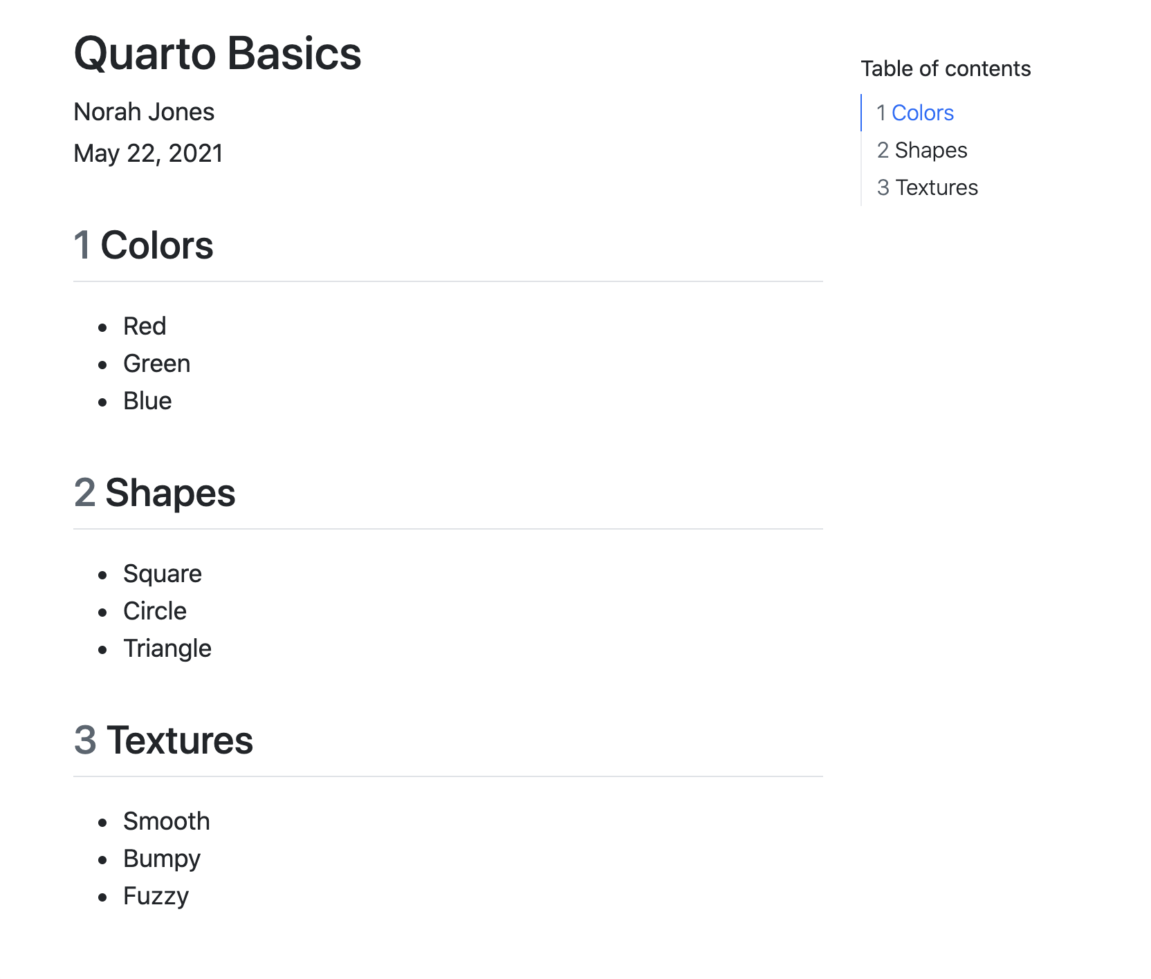
You can use a table of contents and/or section numbering to make it easier for readers to navigate your document. Do this by adding the toc and/or number-sections options to document options. Note that these options are typically specified at the root level because they are shared across all formats.

---
title: Quarto Basics
author: Norah Jones
date: 'May 22, 2021'
toc: true
number-sections: true
---

## Colors

- Red
- Green 
- Blue

## Shapes

- Square
- Circle
- Triangle

## Textures

- Smooth
- Bumpy
- Fuzzy

Here’s what this document looks like when rendered to HTML.

There are lots of options available for controlling how the table of contents and section numbering behave. See the output format documentation (e.g. HTML, PDF, MS Word) for additional details.

Equations

You can use LaTeX equations within markdown.

Einstein's theory of special relatively that expresses the equivalence of mass and energy:

$E = mc^{2}$

This appears as follows when rendered.

Einstein’s theory of special relatively that expresses the equivalence of mass and energy:

$E = mc^{2}$

Inline equations are delimited with $…$ . To create equations in a new line (display equation) use $$…$$. See the documentation on markdown equations for additional details.

Citations

To cite other works within a Quarto document. First create a bibliography file in a supported format (BibTeX or CSL). Then, link the bibliography to your document using the bibliography YAML metadata option.

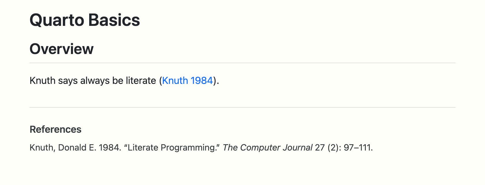
Here’s a document that includes a bibliography and single citation.

---
title: Quarto Basics
format: html
bibliography: references.bib
---

## Overview

Knuth says always be literate [@knuth1984].

## References

Contents of references.bib

references.bib

@article{knuth1984,
  title={Literate programming},
  author={Knuth, Donald E.},
  journal={The Computer Journal},
  volume={27},
  number={2},
  pages={97--111},
  year={1984},
  publisher={British Computer Society}
}

Note that items within the bibliography are cited using the @citeid syntax.

 Knuth says always be literate [@knuth1984].

References will be included at the end of the document, so we include a ## References heading at the bottom of the source file.

Here is what this document looks like when rendered.

Rendered document with references section at the bottom the content of which reads 'Knuth, Donald E. 1984. Literate Programming. The Computer Journal 27 (2): 97-111.'

The @ citation syntax is very flexible and includes support for prefixes, suffixes, locators, and in-text citations. See the documentation on Citations to learn more.

Cross References

Cross-references make it easier for readers to navigate your document by providing numbered references and hyperlinks to figures, tables, equations, and sections. Cross-reference-able entities generally require a label (unique identifier) and a caption.

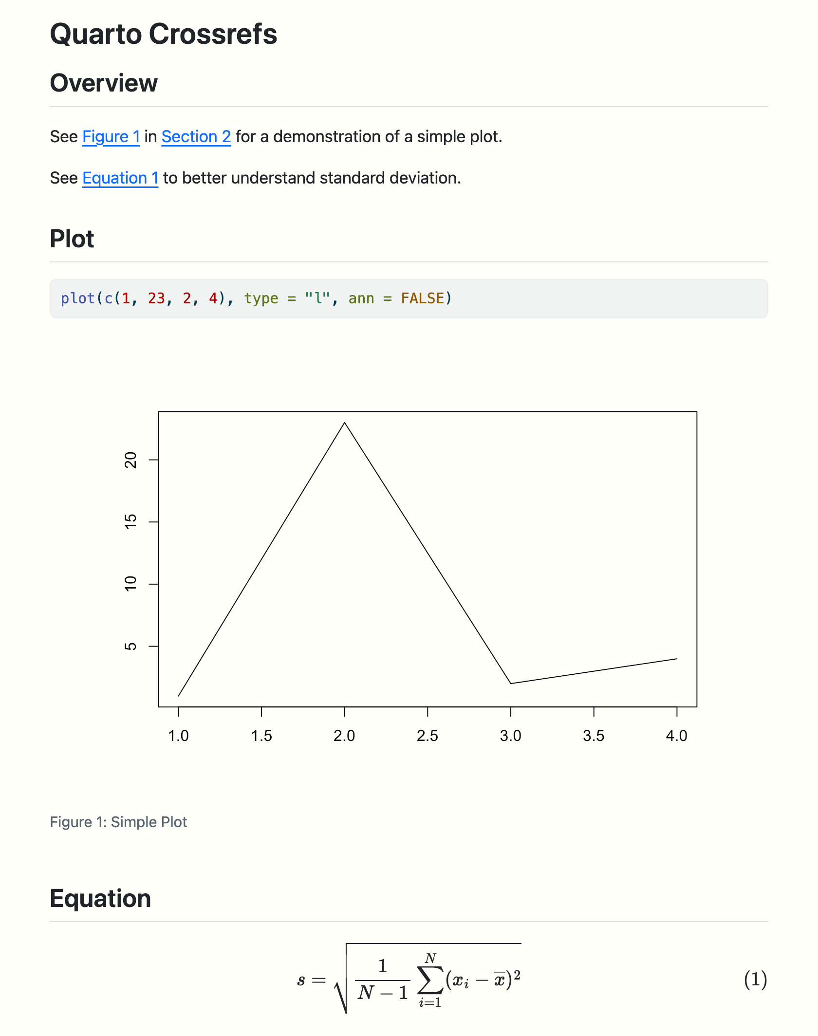
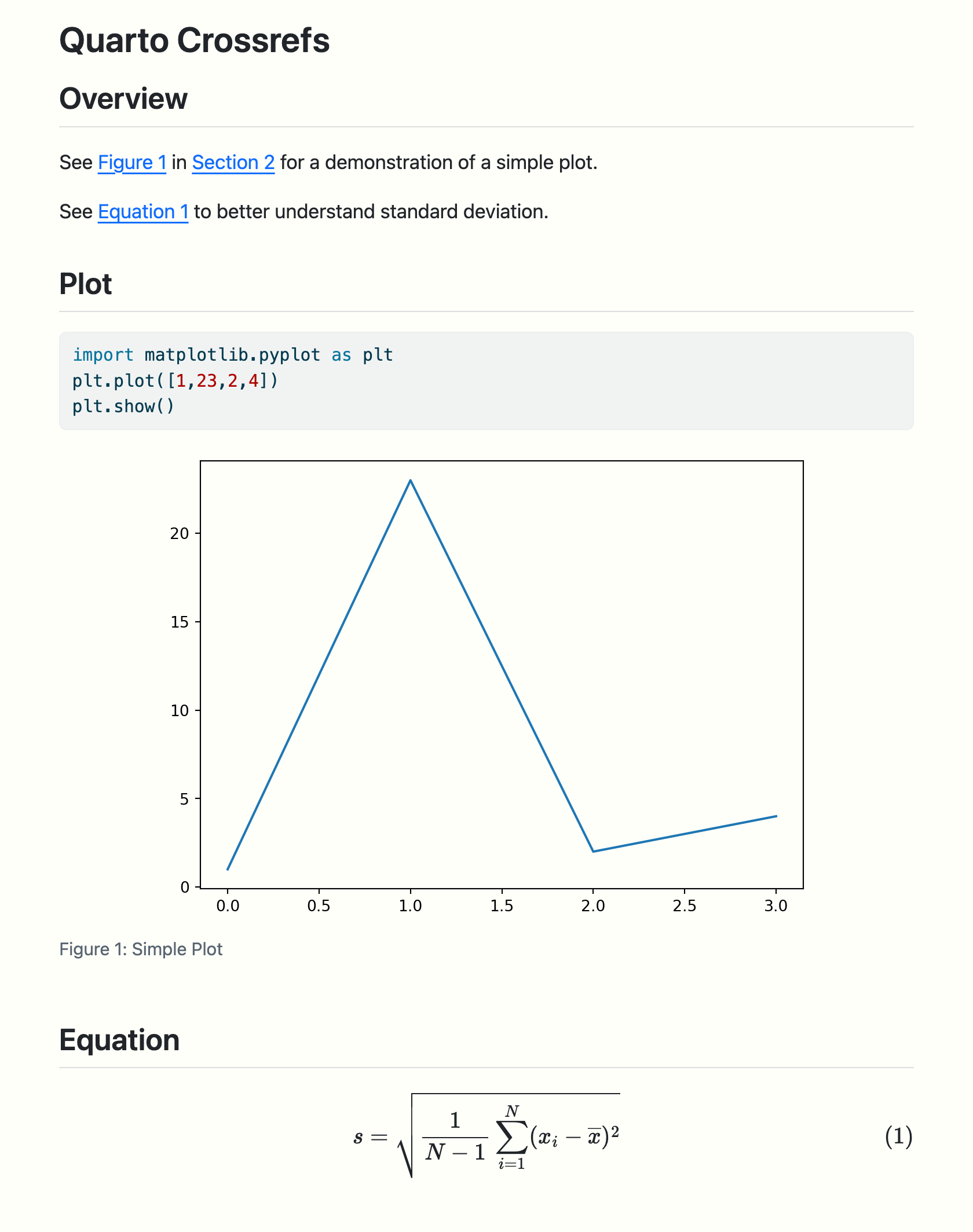
This example illustrates cross-referencing various types of entities.

R
Python

---
title: Quarto Crossrefs
format: html
---

## Overview

See @fig-simple in @sec-plot for a demonstration of a simple plot. 

See @eq-stddev to better understand standard deviation.

## Plot {#sec-plot}

```{r}
#| label: fig-simple
#| fig-cap: "Simple Plot"
plot(c(1, 23, 2, 4), type = "l", ann = FALSE)
```

## Equation {#sec-equation}

$$
s = \sqrt{\frac{1}{N-1} \sum_{i=1}^N (x_i - \overline{x})^2}
$$ {#eq-stddev}

---
title: Quarto Crossrefs
format: html
---

## Overview

See @fig-simple in @sec-plot for a demonstration of a simple plot. 

See @eq-stddev to better understand standard deviation.

## Plot {#sec-plot}

```{python}
#| label: fig-simple
#| fig-cap: "Simple Plot"
import matplotlib.pyplot as plt
plt.plot([1,23,2,4])
plt.show()
```

## Equation {#sec-equation}

$$
s = \sqrt{\frac{1}{N-1} \sum_{i=1}^N (x_i - \overline{x})^2}
$$ {#eq-stddev}

We cross-referenced sections, figures, and equations. The table below shows how we expressed each of these.

Entity	Reference	Label / Caption
Section	`@sec-plot`	ID added to heading: `# Plot {#sec-plot}`
Figure	`@fig-simple`	YAML options in code cell: `#\| label: fig-simple #\| fig-cap: "Simple Plot"`
Equation	`@eq-stddev`	At end of display equation: `$$ {#eq-stddev}`

And finally, here is what this document looks like when rendered.

R
Python

Rendered page with linked cross references to figures and equations.

See the article on Cross References to learn more, including how to customize caption and reference text (e.g. use “Fig.” rather than “Figure”).

Callouts

Callouts are an excellent way to draw extra attention to certain concepts, or to more clearly indicate that certain content is supplemental or applicable to only some scenarios.

Callouts are markdown divs that have special callout attributes. To create a callout within a markdown cell, type the following in your document.

::: {.callout-note}
Note that there are five types of callouts, including:
`note`, `tip`, `warning`, `caution`, and `important`.
:::

This appears as follows when rendered.

Note

Note that there are five types of callouts, including note, tip, warning, caution, and important.

You can learn more about the different types of callouts and options for their appearance in the Callouts documentation.

Article Layout

The body of Quarto articles have a default width of approximately 700 pixels. This width is chosen to optimize readability. This normally leaves some available space in the document margins and there are a few ways you can take advantage of this space.

In this example, we use the reference-location option to indicate that we would like footnotes to be placed in the right margin.

We also use the column: screen-inset cell option to indicate we would like our figure to occupy the full width of the screen, with a small inset.

R
Python

---
title: Quarto Layout
format: html
reference-location: margin
---

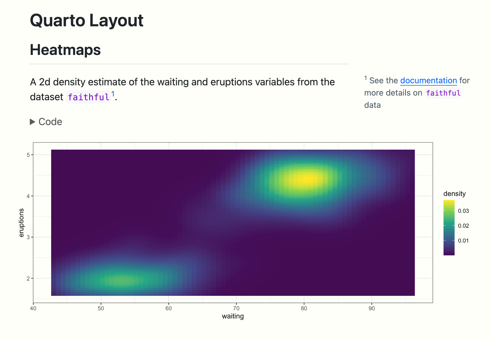
## Heatmaps

A 2d density estimate of the waiting and eruptions variables from the dataset `faithful`^[See the [documentation](https://rdrr.io/r/datasets/faithful.html) for more details on `faithful` data].

```{r}
#| code-fold: true
#| column: screen-inset
#| fig-width: 10
#| fig-height: 4
library(ggplot2)

ggplot(faithfuld, aes(x = waiting, y = eruptions, fill = density)) +
  geom_tile() +
  scale_fill_viridis_c() +
  theme_bw()
```

---
title: Quarto Layout
format: html
reference-location: margin
---

## Heatmaps

A 2d density estimate of the waiting and eruptions variables from the dataset `faithful`^[See the [documentation](https://rdrr.io/r/datasets/faithful.html) for more details on `faithful` data].

```{python}
#| code-fold: true
#| column: screen-inset
from plotnine import *
from plotnine.data import faithfuld

(
  ggplot(faithfuld, aes(x='waiting', y='eruptions', fill='density'))
  + geom_tile()
  + theme_bw()
  + theme(figure_size=(10, 4))
) 
```

Here is what this document looks like when rendered.

Document with Quarto Layout title at the top followed by Heatmaps header with text below it. Next to the text is a footnote in the page margin. Below the text is a toggleable code widget to hide/reveal the code followed a wide plot that extends into the right margin.

You can locate citations, footnotes, and asides in the margin. You can also define custom column spans for figures, tables, or other content. See the documentation on Article Layout for additional details.

Learning More

You’ve now learned the basics of using Quarto! Once you feel comfortable creating and customizing documents here are a few more things to explore:

Presentations — Author PowerPoint, Beamer, and Revealjs presentations using the same syntax you’ve learned for creating documents.
Websites — Publish collections of documents as a website. Websites support multiple forms of navigation and full-text search.
Blogs — Create a blog with an about page, flexible post listings, categories, RSS feeds, and over twenty themes.
Books — Create books and manuscripts in print (PDF, MS Word) and online (HTML, ePub) formats.
Interactivity — Include interactive components to help readers explore the concepts and data you are presenting more deeply.

Additionally, if you are interested in seeing how to use Quarto from within .ipynb notebooks, check out the documentation on using the Positron Notebook Editor with Quarto.